Matemathics Explanations of Plot Programming
Math Explanation CODE relations
From Andraelity, how CODE using math.
In thy following lines we are going to verify or create the connexion that would allow us to unite code with mathematics
Shaders-PLANE-PolyG
We already had stablish ideas that are very important on regards, of how it is to paint shapes that are define by mathematical rules.
This rules that we could make use to present more and more particularities on regards on the uses of programming properties, but over all
Mathematical properties, ideas an concepts, that are generaly define with mathematical properties.
Now the main ideas on painting were define, the next thing that we need to specify is how we could make modification on this shapes
over the space, lets explain.
Index Webpages Redirect
- &. Index
- 0. EulersIdentity
- 1. Derivatives
- 2. Shaders
Computer Shaders Graphics
Triangle Rotation.

$$\begin{aligned}
&\text{First of all we need to identify two types of rotation:}\\
&\mathbf{1.\ Rotation\ on\ its\ axis}\\
&\mathbf{2.\ Rotation\ on\ a\ point}\\
\end{aligned}$$
float2x2 rotationMatrix(float rotationAngle)
{
    float2x2 rot = float2x2(cos(rotationAngle),
                            -sin(rotationAngle),
                                                sin(rotationAngle),
                                                cos(rotationAngle));

    return rot;
}
$$\begin{aligned}
&\mathbf{1.\ Rotation\ on\ its\ axis}\\
\end{aligned}$$
fixed4 frag (PixelData i) : SV_Target
{


float2 uv =  i.uv ;

float4 colorWhite = float4(1,1,1,1); // Color white.
float4 colorBlack = float4(0,0,0,1); // Color Black.

float2 coordinateScale = (uv * 2.0)  - 1.0;

float2 size = float2(0.5 ,0.5);
float2 screenSpace = coordinateScale;

float2x2 matrixOut = rotationMatrix(_Time.y);
screenSpace = mul(matrixOut, screenSpace);

float disHypotenuse = dot(size, screenSpace ) - (size.x * size.y);

screenSpace = -screenSpace;

float sdf = max(max(screenSpace.x, screenSpace.y), disHypotenuse);

float shader = 1.0 - smoothstep(0.0, 0.01, sdf);

float4 col = colorBlack;

col = fixed4(shader, shader, shader, 1.0);

return col;

}
$$\begin{aligned}
&\mathbf{2.\ Rotation\ on\ a\ point}\\
\end{aligned}$$
fixed4 frag (PixelData i) : SV_Target
{


float2 uv =  i.uv ;

float4 colorWhite = float4(1,1,1,1); // Color white.
float4 colorBlack = float4(0,0,0,1); // Color Black.

float2 coordinateScale = (uv * 2.0)  - 1.0;

float2 size = float2(0.5 ,0.5);

float2 position = float2(0.5, 0.5);

float2x2 matrixOut = rotationMatrix(_Time.y);

position = mul(matrixOut, position);
float2 screenSpace = coordinateScale - position;

float disHypotenuse = dot(size, screenSpace ) - (size.x * size.y);

screenSpace = -screenSpace;

float sdf = max(max(screenSpace.x, screenSpace.y), disHypotenuse);

float shader = 1.0 - smoothstep(0.0, 0.01, sdf);

float4 col = colorBlack;

col = fixed4(shader, shader, shader, 1.0);

return col;

}
$$\begin{aligned}
&\textbf{1. Represent the Point in Polar Coordinates}\\
&\text{Any point}\ (x, y) \text{can be described by its distance from the origin }(r)\\
&\text{and its current angle } (\theta):\\
&x = r \cos \theta \\
&y = r \sin \theta\\
&\\[-15pt]\\
&\textbf{2. Apply the Rotation} \\
&\text{Now, we rotate the point by an additional angle}\ \phi.\\
&\text{The distance $r$ stays the same, but the new angle is} \ (\theta + \phi).\\
&\text{The new coordinates } (x', y')\ \text{are}\ :\\
&x' = r \cos(\theta + \phi)\\
&y' = r \sin(\theta + \phi)\\
&\\[-15pt]\\
&\textbf{3. Use Trigonometric Identities }\\
&\text{We apply the angle addition formulas:}\\
&\cos(A + B) = \cos A \cos B - \sin A \sin B\\
&\sin(A + B) = \sin A \cos B + \cos A \sin B\\
&\text{Substituting these into our equations for } x' and \ y':\\
&x' = r(\cos \theta \cos \phi - \sin \theta \sin \phi)\\
&y' = r(\sin \theta \cos \phi + \cos \theta \sin \phi)\\
&\\[-15pt]\\
&\textbf{4. Final Substitution}\\
&\text{By distributing }\ r \ \text{and substituting the original }\\
&x = r \cos \theta \\
&and \\
&\ y = r \sin \theta \\
&\text{ back into the equations, we get the standard rotation transformation:}\\
&x' = x \cos \phi - y \sin \phi \\
&y' = x \sin \phi + y \cos \phi \\
&\\[-15pt]\\
&\textbf{5. Form the Matrix}\\
\\
&\text{We can write these two linear equations as a single matrix multiplication:}\\
&\begin{pmatrix} x' \\ y' \end{pmatrix} = \begin{pmatrix} \cos \phi & -\sin \phi \\ \sin \phi & \cos \phi \end{pmatrix} \begin{pmatrix} x \\ y \end{pmatrix}\\
\\
&\text{This gives us the standard Rotation Matrix:}\\
&R(\phi) = \begin{pmatrix} \cos \phi & -\sin \phi \\ \sin \phi & \cos \phi \end{pmatrix}\\
\\
&\text{But on HLSL and CG Programing the order of an array is Column Major:}\\
&\mathbf{column\ Major\ }R(\phi) = \begin{pmatrix} \cos \phi & \sin \phi \\ -\sin \phi & \cos \phi \end{pmatrix}\\
\end{aligned}$$
$$\begin{aligned}
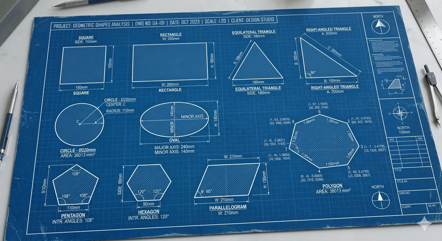
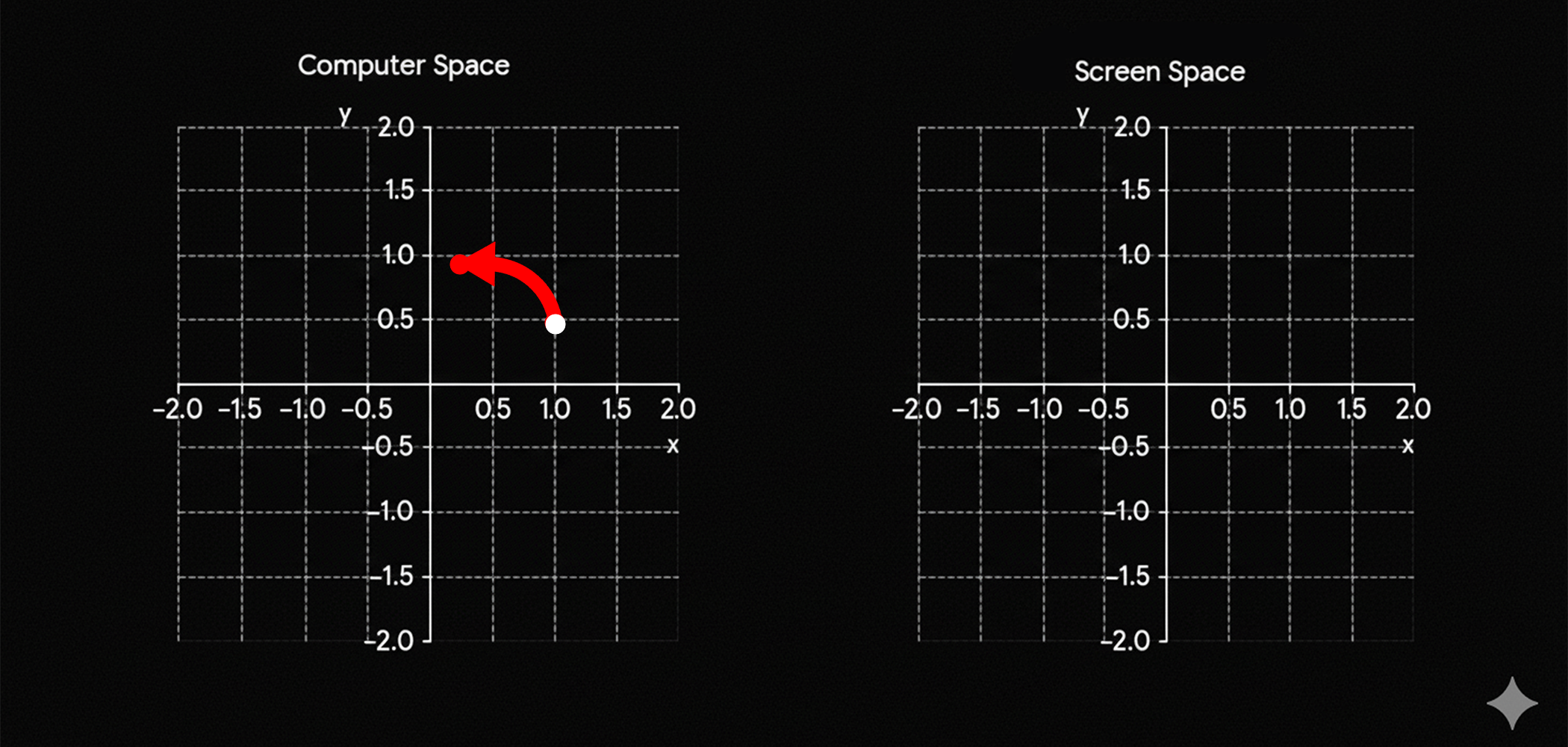
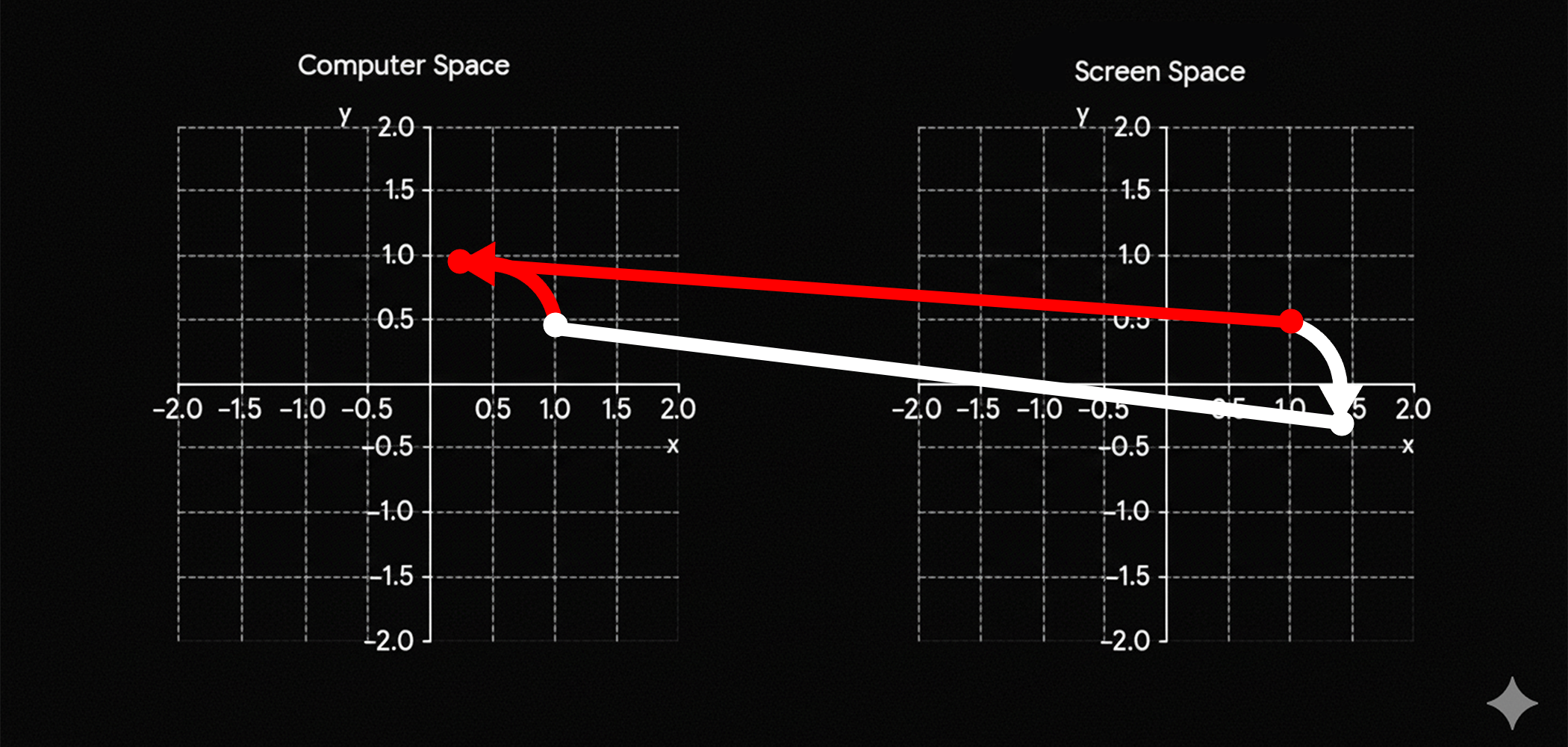
&\text{if you are noticing that the rotation of the shape happens in a clockwise notation. }\\
&\text{but the points are rotating according to the formula are rotating in the counter-clock wise}\\
&\text{direction}\\
&\text{why ????????}\\\
\end{aligned}$$
$$\begin{aligned}
&\text{The reason why is because we are rotating the plane not the shape.}\\
&\text{The idea happens to beside in the same explanation of the ScreenSpace and the ComputationSpace}\\
&\text{if you rotate the points in the ComputationSpace are going to be presented in the}\\
&\text{ScreenSpace differently.}\\
&\text{}\\\
\end{aligned}$$
$$\begin{aligned}
&\text{The idea is that every point is going to be modify in the computer space, but cuz this }\\
&\text{points are also part of the screenspace is when you are going to notice that the }\\
&\text{information is going to be represented in a completely different rotation, thanks to }\\
&\text{this representation.}\\
\end{aligned}$$
Shader_RotationExplain_1
Shader_RotationExplain_2
Scalation
$$\begin{aligned}
&\text{The scalation is pretty straigh forward, what we need to scale is the plane;}\\
&\text{not the shape, by the scalation of the plane we are going to also scale the shape }\\
&\text{which is going to be present in the plane, cuz obviously the shape is in the plane.}\\
\end{aligned}$$
$$\begin{aligned}
&\text{The shape that we are going to scale in this case is going to be the triangle, this}\\
&\text{this shape contains multiple expressions in regards of mathematical theories, and }\\
&\text{also at the same time really simple to imagine, the idea here is to think as if the}\\
&\text{measurements, or more specificly the units that make the measurement space measure }\\
&\text{something else. }\\
\end{aligned}$$
fixed4 frag (PixelData i) : SV_Target
{

    float2 uv =  i.uv ;

    float4 colorWhite = float4(1,1,1,1); // Color white.
    float4 colorBlack = float4(0,0,0,1); // Color Black.

    float2 coordinateScale = (uv * 2.0)  - 1.0;
    coordinateScale = coordinateScale/(float2(0.55555, 1.0));

    float2 size = float2(0.5 ,0.5);
    float2 screenSpace = coordinateScale;
    float scalationRatio = 2.0;

    screenSpace = scalationRatio * coordinateScale;
    float disHypotenuse = dot(size, screenSpace ) - (size.x * size.y);

    screenSpace = -screenSpace;

    float sdf = max(max(screenSpace.x, screenSpace.y), disHypotenuse);

    float shader = 1.0 - smoothstep(0.0, 0.01, sdf);

    float4 col = colorBlack;

    col = fixed4(shader, shader, shader, 1.0);

    return col;

}
$$\begin{aligned}
&\text{In this case we can identify that the entire idea of SCALATION could be summarize in 2 lines}\\
&\text{the uses of the scalation is summarize as a relation of how many unit of measure we can fit}\\
&\text{in the minimum entity of measure, its like saying, how many ones we can fit in one one if we make}\\
&\text{ one half equal to 1}\\
&\text{ }\\
\end{aligned}$$
$$\mathbb{R} = \mathbf{Real \ numbers }\\$$
$$\text{if we make this relationship for a set of real number } \\$$
$$\\[5ex]\\$$
$$scale = \frac{1}{2}$$
$$\\[5ex]\\$$
$$\mathbb{R}_{\text{spaceScale}} = \quad \mathbb{R} * scale \quad = \quad \mathbb{R} * \frac{1}{2}\\$$
$$\\[5ex]\\$$
$$\text{but we want to make such relation that makes } \\$$
$$\\[5ex]\\$$
$$\mathbb{R}_{\text{spaceScale}} \implies \mathbb{R} * \frac{1}{2} = \mathbb{R} * 1.0\\$$
$$\\[5ex]\\$$
$$\text{which is false, there is no way to make sense of the previous equation, its just not true} \\$$
$$\text{so instead we create a different space that allows to make the prevoius space true} \\$$
$$\text{then for another set of real numbers we make the next relationship to make sense of both spaces } \\$$
$$\\[5ex]\\$$
$$\mathbb{R}_{\text{spaceCorrection}} \implies \frac{1}{\mathbb{scale}} * \mathbb{R}_{\text{spaceScale}}$$
$$\\[5ex]\\$$
$$\mathbb{R}_{\text{spaceCorrection}} \implies \frac{1}{\mathbb{scale}} * \mathbb{R}_{\text{spaceScale}} = 2.0 * \mathbb{R}_{\text{spaceScale}} = \mathbb{R} * 1.0\\$$
$$\\[5ex]\\$$
$$\begin{aligned}
&\text{How many 1's or units in the first space , } \implies \frac{2}{1} = 2\\
&\text{are in 1's or units of the base space? }\\
\end{aligned}$$
$$\text{What we can conclude is that there are 2 units in the first space } \\$$
$$\text{for each unit of the base space}\\$$
$$\\[5ex]\\$$
$$\text{How many } \mathbb{R}_{\text{spaceScale}} \quad \text{in} \quad \mathbb{R}? ,
\implies \frac{\mathbb{R}_{\text{spaceScale}}}{\mathbb{R}} = scale$$
$$\\[5ex]\\$$
$$\frac{\mathbb{R}_{\text{spaceScale}}}{\mathbb{R}} = \quad \frac{\mathbb{\mathbb{R} * scale}}{\mathbb{R}} \quad = \quad scale$$
float scalationRatio = 2.0;

screenSpace = scalationRatio * coordinateScale;